What am I up to

Read part 1 here

This blogpost is a rework of my old post from medium.com. You can find the original post here

Ten years ago, Fabien Sanglard wrote an article about the “business card raytracer” — a very short C++ code that generates a full raytraced image with advanced effects. I remade the code in python, and it worked comparably fast, although it wasn’t short anymore. Now, I could play with the code and tweak it. So I decided to take it one step further and create not just a picture but an entire animation.

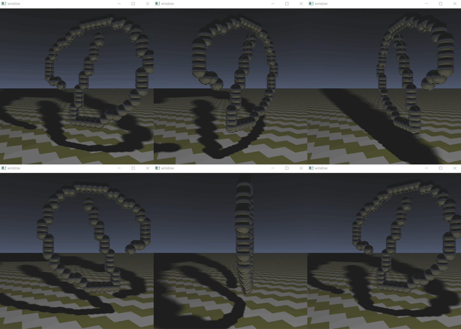
In part 1, I explained the original code and my first porting attempt. In this part, I will describe how I made the animation. In the end, it is a single geometric formula, but getting to it is hard. So we will talk about the math used by the code. Namely, I will:

• First, explain how the original code defined the location of the spheres in 3D space,
• Then, use trigonometry to derive a formula for rotating the spheres in 3D with each frame,
• Finally, patch the code to implement the rotation formula, and make use of OpenCV to show the results,

In the end, I will share a link to the code, so you can play with it too!

Why did I do it, anyway?

Because it is fun to take a toy and disassemble it to see how it works. And now, that I understand how it works,

it is twice as fun tweaking the toy to change what it does.

In the previous episode

Let me tell you what we are dealing with. We have a code in python that renders an image of a logo, consisting of spheres, with the floor with the sky in the background. The code uses ray casting (and dirty hacks).

See part 1 to read more about how the code works. Briefly, the “camera” cast rays through each pixel of a virtual 2D “screen”. Each ray either hits the floor, the sky, or a sphere. The code finds what is hit and renders a pixel of the floor or sky colour if one of them is hit. If the ray hits a sphere, the ray is bounced, and the ray casting is continued until the sky or the floor is hit.

Making animation

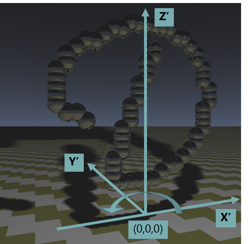
My plan to animate the generated image was to make it rotate somewhere around the middle on the X-axis (more on the axes placement later):

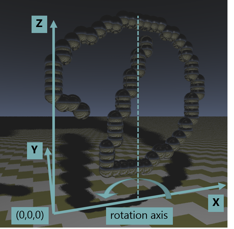
To make the animation work, I wanted to move the spheres in the rendered 3D space. Thus, I needed to understand how the coordinates of the spheres were encoded in the original code.

Where are the spheres?

The position of the spheres was fixed in the original code on a 2D plane. The code defined a variable G, which was a 2D byte array, describing a mask of where spheres must be located on some imaginary 2D plane:

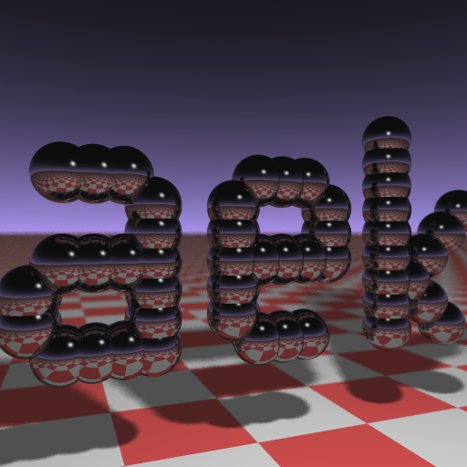
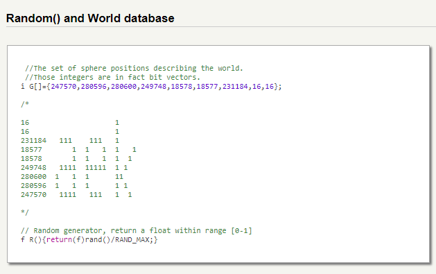
But our final image is definitely 3-dimensional. So, how does this 2D mask define the location of the spheres in our imaginary 3D space? Where is this 2D plane located?

After some investigation, I found that coordinates were hardcoded inside the ‘tracer’ function. This function casts a ray and checks whether the ray hits any sphere. Its code implements the formula from here — see page 7, geometric proficiency is required (I also included a deck in GitHub repo, explaining how it works):

Here is how it works. First, the code checks every bit in mask G, iterating over indices k and j (lines 39–41). As mentioned above, it must equal “1” for a sphere to be plotted — or, in python terms, it must be True (line 41). If this bit is True, then there is a sphere on the 2D plane. The calculation in line 42 shows that this sphere will be placed at the 3D coordinates (k, 0, j+4). The sphere radius is always set to 1, and its square, which is also 1, is used later in line 44.

How does this look in 3D?

Y-coordinate is 0 for all the spheres. This defines the 2D surface, I was searching for. All the spheres are rendered on the imaginary 2D plane located at Y=0, while X and Z axes define the column and the row for each sphere, respectively (starting at 0 for columns and at 4 for rows, and increasing by 1 for each row/column):

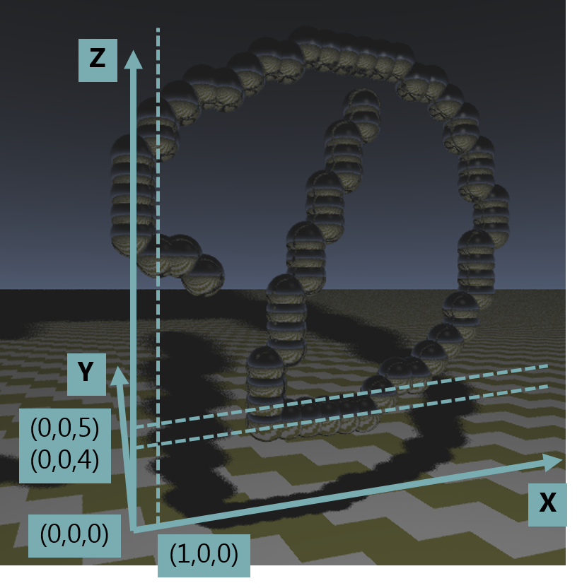
Now I knew which coordinates the spheres had in 3D space. But how do I alter these coordinates on each frame to have an animation?

The math

To describe the rotation, I first set a new coordinate system (X’, Y’, Z’), where it would be easier to do. All its axes will be parallel to the original ones, but they are placed in such a way that Z’ is the rotation axis:

I chose to create 120 frames. If we look top-down on the picture, that’s what we would want to see on different frames:

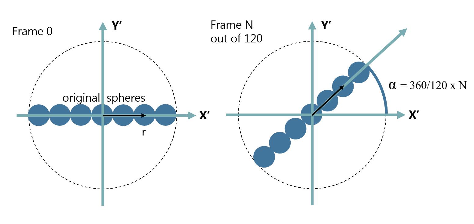
Let’s look at a single sphere whose center is r units away from the rotation center on frame 0. For the frame N, I would have to change the X’ and Y’ coordinates of this sphere from (r, 0) to (r x cos(alpha), r x sin(alpha)). So, in the new coordinate system (X’, Y’, Z’), the coordinates of this sphere on the frame N would be:

x = r x cos(alpha)
y = r x cos(alpha)

In the original coordinate system (X, Y, Z), the coordinates of this sphere on the frame N would therefore be:

x = rotation center x + r x cos(alpha)
y = rotation center y + r x cos(alpha)

where

rotation center y = 0 (all the spheres were at Y=0)

and

rotation center x = some function of(number of spheres columns)

These are the coordinates I was looking for.

The code

Now I could calculate the new coordinates:

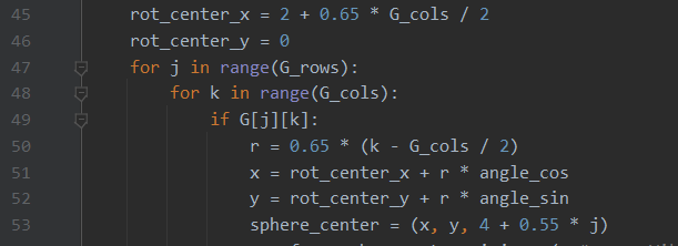
This code, as before, iterates over the 2D mask G (lines 47–49). But now, I generate 3D coordinates for each sphere dynamically. On lines 45–46, I define two out of three coordinates, and it defines a line in 3D space, which will be our rotation axis. Its y coordinate is 0, while x coordinate points approximately to the middle of all the spheres on the X-axis, as described above. Then, for each present sphere, the abovementioned distance r is calculated on line 50. Finally, we calculate the position of each sphere for the given frame using the sin and cos of the angle corresponding to the frame on lines 51–53.

Sidenote: You might notice a magical constant of 0.55 that appears and adjusts the Z-axis coordinate on line 53. It comes up because of other changes I have introduced behind the scene to adjust the image scale. You can safely ignore it.

The result

After waiting for about 6.5 minutes, I have finally got my frames rendered. All that was left was to add some boilerplate code that would render them one after another. I used OpenCV for python and its method cv2.imshow() to render the images cyclically:

and it worked!

To wrap it up, I have polished and annotated the code with docstrings, comments, and type hints. The resulting code is more than 18500 symbols. This would not fit on a business card, unfortunately. But hey, now you can actually read and understand the code, and you don’t have to be a professional C++ developer to do so!

What can you do with all of this?

• You can find the code on my GitHub, download it, run it, and play with it. The code should be possible to follow even if you are a junior python developer.
• You can change the logo, generate an animation with your own initials, and have fun because you too understood how to disassemble a toy and change what it does.
• You can tweak the code more and improve what it does even further. Like I did by adding animation capability. How about coloured spheres, for example?
• Or maybe you just enjoyed reading this post and learned something new about the math of 3D rendering.
• Finally, there is also a PowerPoint presentation that you can read to understand how the ‘tracer’ code works if you feel ready to go through a challenging sketch of the proof.